- Day 1: What is CPU Scheduling? -
CPU Scheduling.
CPU Scheduling is a method used within Operating Systems. This method decides which process in
the ready queue gets CPU Time.
As CPU's can only handle one task at a time, this is essential for maximizing CPU utilization
and
minimizing response and wait times for processes.
Definitions
Process: An active execution of a program running on an Operating System.
Thread: The smallest sequence of manageable programmed instructions.
Scheduler: A software component of an operating system, that decides what process, thread, or task should run next on the CPU.
Context Switch: A mechanism used by operating systems to save a current state of a running process or thread, then loads a state of another process or thread.
Throughput: The actual data rate that is transmitted or processed within a specific time frame. Often expressed in bits per second.
Latency: The time delay between initiation of an action and receiving a corresponding response. Often measured in milliseconds.
CPU Scheduling uses a ready queue, in that processes are served from. This is an important function of CPU's as they can only handle a single task at a time, and there tends to be multiple running tasks at any given time that need to be processed. This also ensures whenever the CPU is idle, the Operating System has at least a single process available in the ready queue.
The internal mechanisms of the Scheduler ensure all processes are handled appropriately based upon the underlying algorithm to ensure maximum throughput and minimal latency between tasks. Optimal performance from these algorithms aim to keep the CPU busy at all times.
There are two main types of scheduling methods, preemptive scheduling and non-preemptive scheduling. Preemptive scheduling is when a process switches from a running state to a ready state or from a waiting state to a ready state, where non-preemptive scheduling is used when a process terminates, or when a process switches from a running state to waiting state and only reassigns when that process is complete. With preemptive scheduling the scheduler may decide depending on the algorithm in use, to use context switching and stop a current process, before switching to the next process in the queue. The scheduler tends to operate at the thread level treating each thread as an independently scheduled unit within a process.
- Day 2: First Come First Served -
FCFS Scheduling.
This algorithm follows the First-In, First-Out (FIFO) principle. It's non-preemptive, and once a
process
starts, it will run until completion, without interruption.
How it Works
First Come First Served is a Scheduling Algorithm that works as it is defined, when a process arrives into the ready queue, it is served in the order it comes in, until completion. Due to it being non-preemptive, the order does not utilize Preemptive Context Switching, and instead initializes, and runs, a single process, until completion.
Advantages
First Come First Served, is simple to implement, it's an easier to design and understand scheduling algorithm and has minimal overhead. It simply runs the processes in the order they arrive, due to this it has what could be considered a fair execution order, as processes are handled in a first-in first-out condition. Thanks to this, every process should eventually execute, with predictable behavior. Allowing for easier analysis of performance conditions.
Disadvantages
Disadvantages to First Come First Served are wait time, response time, and poor handling of urgency. As each process is treated equally regardless of priority, length, interaction requirements, or deadlines. The wait time, and response times, end up being linear. With Process A and Process B arriving at the same time, in a case where Process A has a wait time of 0ms, due to it arriving first, but a completion time of 20ms, leading to Process B, having a wait time of 20ms, in addition to it's completion time. These times can become unnecessarily large, leading to sluggish systems with high latency.
Convoy Effect
In alignment with disadvantages, the Convoy Effect is known to be the biggest weakness of First Come First Served Scheduling as a long running process at the front of the queue ensures all shorter processes are required to wait. In the example of Process A having a completion time of 20ms assume Process B has a completion time of 10ms, and a third, Process C with a completion time of 5ms, if Process A arrives before B then C, the total time to execute Process C will be 35ms. Process C having to wait until Process B and Process A execute fully, despite needing the least amount of processing time on the CPU.
Exercise
Mathematically if we pick 5 Processes, with random execution times by rolling a d20 dice, and multiplying by 10 to ensure we have substantial data. We can chart the processes in a quick exercise. With the expression Process => Completion Time from Arrival.
Exercise A
P1 - 40ms P2 - 60ms P3 - 130ms P4 - 30ms P5 - 170ms
P1 => 40ms, P2 => 100ms, P3 => 230ms, P4 => 260ms, P5 => 430ms
Exercise B
P1 - 160ms P2 - 40ms P3 - 100ms P4 - 150ms P5 - 50ms
P1 => 160ms, P2 => 200ms, P3 => 300ms, P4 => 450ms, P5 => 500ms
Exercise C
P1 - 20ms P2 - 10ms P3 - 160ms P4 - 80ms P5 - 80ms
P1 => 20ms, P2 => 30ms, P3 => 190ms, P4 => 270ms, P5 => 350ms
- Day 3: Shortest Job First -
SJF Scheduling.
Shortest Job First Scheduling, is a scheduling algorithm, that finds the process with the
shortest burst time (execution time) and selects it to run next in the ready queue.
How it works
With Non-Preemptive SJF Scheduling, the scheduler or scheduling algorithm looks at all available processes, and picks the one with the shortest burst time. After the process runs until completion, the next shortest burst time process is selected. In the case multiple processes have the same burst time, they are scheduled using FCFS Scheduling.
Advantages
The advantages to Shortest Job First Scheduling are in relation to the minimal wait times provided by this algorithm. As well as being simple and easy to implement (minus not knowing burst times in advance). It's an optimal algorithm for minimizing wait times, and is useful for batch processing.
Disadvantages
In the case of Preemptive Shortest Job First Scheduling, longer processes may never get CPU time in the case shorter processes keep arriving in the queue, while this can be mitigated by using priority or aging, in a Non-Preemptive SJF Schedule CPU Starvation is still possible as well, however is more apparent in Preemptive SJF. Additionally, burst times are often unknown in advance, so estimation is required.
Exercise
For the example, we'll be looking at Non-Preemptive Shortest Job First Scheduling in order to compare it against First Come First Serve Scheduling. Using the same processes, after we'll compare the two. As before Process => Completion Time from Arrival.
Exercise A
P1 - 40ms P2 - 60ms P3 - 130ms P4 - 30ms P5 - 170ms
P4 => 30ms, P1 => 70ms, P2 => 130ms, P3 => 260ms, P5 => 430ms
Exercise B
P1 - 160ms P2 - 40ms P3 - 100ms P4 - 150ms P5 - 50ms
P2 => 40ms, P5 => 90ms, P3 => 190ms, P4 => 340ms, P1 => 500ms
Exercise C
P1 - 20ms P2 - 10ms P3 - 160ms P4 - 80ms P5 - 80ms
P2 => 10ms, P1 => 30ms, P4 => 110ms, P5 => 190ms, P3 => 350ms
Comparison
With first come first serve, we can see regardless of the burst time, the process arrives and is executed in the order received. Without priorities we can't determine if it's successfully executing urgent processes in a timely manner, but the same goes for shortest job first. The main difference here is the optimization that processes with a short burst time are executed first, without having an extensive wait time.
For that, we can see this reflect in Exercise 3 from both Day 2 and Day 3, for P1: 20ms, P2: 10ms, P3: 160ms, P4: 80ms, P5: 80ms. For first come first serve, P4 and P5 have a wait time of 190ms for P4, and 270ms for P5. Where shortest job first has a wait time of 30ms for P4, and 110ms for P5. These exercises both focused on arrival order, and execution time, without priority, or context switching. However they also highlight the foundations of CPU Scheduling and the Algorithms in use.
- Day 4: Round Robin Scheduling -
RR Scheduling
Round Robin (RR) is our first fully preemptive scheduling algorithm, it uses time quantum or
time slices, that cycle through the ready queue in circular order. After each process gets its
turn on the CPU, it routes to the next process with preemptive context switching.
How it works
Using time quantum, as a variable in the algorithm, RR cycles through processes in the ready queue until each process is completed. In the simplest process possible, if we use q for time quantum like so, q = 5, then if P1 with a burst time of 20ms, and P2 with a burst time of 45ms, would cycle in the CPU for the respective slice per time quantum, so P1 would run for 4 slices, until completion, and time P2 would run for 9 slices, until completion.
Advantages
With RR the advantages compound against FCFS, and SJF Scheduling. With this algorithm starvation is unlikely, CPU allocation is consistent for each process, response times in interactive systems decrease. Optimization at this level becomes more dependent on the algorithm and use case, with the time quantum determining the utilization of each process, rather than the burst time of each process.
Disadvantages
Adjacent to the advantage of optimization due to time quantums, the disadvantage also appears here. With performance relaying on having an optimal time quantum. As excessive context switching can reduce efficiency of the algorithm. This also may have a greater average turn around time compared to SJF.
Exercise
For this exercise, we'll give 3 example with differing time quantums. One for q = 4, one for q = 6, and one for q = 10. To ensure we have good data to compare, we'll continue using the process sets from previous examples.
Exercise A
P1 - 40ms P2 - 60ms P3 - 130ms P4 - 30ms P5 - 170ms
Exercise A: (Quantum = 4 ms)
| Process | Burst Time | Completion Time | Turnaround Time | Waiting Time |
|---|---|---|---|---|
| P1 | 40 ms | 178 ms | 178 ms | 138 ms |
| P2 | 60 ms | 262 ms | 262 ms | 202 ms |
| P3 | 130 ms | 390 ms | 390 ms | 260 ms |
| P4 | 30 ms | 146 ms | 146 ms | 116 ms |
| P5 | 170 ms | 430 ms | 430 ms | 260 ms |
| Average | 86 ms | 281.2 ms | 281.2 ms | 195.2 ms |
Exercise B
P1 - 160ms P2 - 40ms P3 - 100ms P4 - 150ms P5 - 50ms
Exercise B: (Quantum = 6ms)
| Process | Burst Time | Completion Time | Turnaround Time | Waiting Time |
|---|---|---|---|---|
| P1 | 160 ms | 500 ms | 500 ms | 340 ms |
| P2 | 40 ms | 190 ms | 190 ms | 150 ms |
| P3 | 100 ms | 388 ms | 388 ms | 288 ms |
| P4 | 150 ms | 490 ms | 490 ms | 340 ms |
| P5 | 50 ms | 252 ms | 252 ms | 202 ms |
| Average | 100 ms | 364 ms | 364 ms | 264 ms |
Exercise C
P1 - 20ms P2 - 10ms P3 - 160ms P4 - 80ms P5 - 80ms
Exercise C: (Quantum = 10ms)
| Process | Burst Time | Completion Time | Turnaround Time | Waiting Time |
|---|---|---|---|---|
| P1 | 20 ms | 60 ms | 60 ms | 40 ms |
| P2 | 10 ms | 20 ms | 20 ms | 10 ms |
| P3 | 160 ms | 350 ms | 350 ms | 190 ms |
| P4 | 80 ms | 280 ms | 280 ms | 200 ms |
| P5 | 80 ms | 290 ms | 290 ms | 210 ms |
| Average | 70 ms | 200 ms | 200 ms | 130 ms |
Comparison
Here we can see structural differences in averages and wait times against the process set. Vastly different from the first two algorithms. Where the processes were ran as they entered the ready queue, or where the shortest job times ran first. With Round Robin we can see each process is treated fairly and routed in and out of the ready queue. Increasing overall times comparatively to non-preemptive scheduling.
While this may be more favorable and optimal for interactive systems where multiple tasks are being completed at once, and it limits disadvantages experienced with previous algorithms. It introduces overhead due to increased use of context switching, which can increase turnaround times and reduce efficiency if the quantum time is too small.
- Day 5: Priority Scheduling -
Priority Scheduling
Priority Scheduling functions by using assigned priorities to determine what process should be
executed next. Each process is assigned a priority value, and the scheduler uses the values as
highest to lowest to determine execution order.
Definitions
Aging: The process of gradually increasing the priority of processes that have waited in the ready queue for long time periods.
How it works
With Priority Scheduling, there are two ways it can operate, Preemptively, with newly arrived higher-priority processes interrupting the running process, or Non-Preemptive, where processes run until completion.
Priority can also be assigned statically, or dynamically. With static assignment being assigned once, and never changing. Or dynamic assignment, where the scheduler may increase or decrease priorities based on wait time, CPU usage, I/O Bandwidth, or existing system policies.
Advantages
Advantages exist for both Preemptive, and Non-Preemptive Priority, as well as Static, and Dynamic use cases.
For Preemptive Static Priority Scheduling, execution of Critical/Urgent Tasks have fast response time, and predictable behavior. Meaning Systems are easier to monitor and test on. This is more suited for Real-Time Systems where time is of the essence.
For Preemptive Dynamic Priority Scheduling, the advantages shift to reducing CPU Starvation, adaptive priorities to adjust to System Conditions, and a favorable environment for Multi-User conditions.
With Non-Preemptive Static Priority Scheduling, these advantages take the form of lower overhead, simple implementation, and predictable execution behaviors. All being beneficial for stable system behaviors.
For Non-Preemptive Dynamic Priority Scheduling,There is a focus on lower overhead, reduced starvation, improved throughput, and adaptability to variable workloads. Allowing for a predictable system with multiple options available for work cases.
Disadvantages
Disadvantages also exist for both Preemptive, and Non-Preemptive Priority, as well as Static, and Dynamic use cases.
With Preemptive Static Priority Scheduling, disadvantages begin with starvation, higher overhead due to context switching, and increased complexity. If higher priority processes keep arriving, lower priority processes may never execute, even with aging this becomes problematic due to priority inversion where a low priority process can keep resources locked until completion due to a greater age.
For Preemptive Dynamic Priority Scheduling, the behavior becoming unpredictable but adaptable, it's complexity increases due to continuously adapting conditions, higher overhead, and a need for fine tuning become apparent here. Processes may oscillate between higher and lower priorities if all variables are not adjusted for optimal performance.
With Non-Preemptive Static Priority, disadvantages remain with starvation, response time and wait time become apparent with higher priority or urgent tasks. As a lower priority process may begin running and be unable to shift, or dynamically shift the priority of a more urgent task. This leads to inefficient utilization due to longer running processes blocking important tasks.
Lastly Non-Preemptive Dynamic Priority Scheduling, disadvantages here exist with complexity, and overhead. Where adjustment needs to be fine tuned, or starvation and delays will become apparent.
Exercise
For this exercise, we'll continue to use the process sets from Exercises A, B, and C. Focusing on Non-Preemptive Static Priority. We'll include priority, and a comparison table will be shown to identify key differences in the previous scheduling algorithms.
Exercise A
P1 - 40ms P2 - 60ms P3 - 130ms P4 - 30ms P5 - 170ms
Priority: P3 - 1, P2 - 2, P1 - 3, P5 - 4, P4 - 5
P3 => 130ms, P2 => 190ms, P1 => 230ms, P5 => 400ms, P4 => 430ms
Exercise A
| Process | Burst Time | Completion Time | Turnaround Time | Waiting Time |
|---|---|---|---|---|
| P1 | 40 ms | 230 ms | 230 ms | 190 ms |
| P2 | 60 ms | 190 ms | 190 ms | 130 ms |
| P3 | 130 ms | 130 ms | 130 ms | 0 ms |
| P4 | 30 ms | 430 ms | 430 ms | 400 ms |
| P5 | 170 ms | 400 ms | 400 ms | 230 ms |
| Average | 86 ms | 276 ms | 276 ms | 190 ms |
Exercise B
P1 - 160ms P2 - 40ms P3 - 100ms P4 - 150ms P5 - 50ms
Priority: P4 - 1, P3 - 2, P1 - 3, P2 - 4, P5 - 5
P4 => 150ms, P3 => 250ms, P1 => 410ms, P2 => 450ms, P5 => 500ms
Exercise B
| Process | Burst Time | Completion Time | Turnaround Time | Waiting Time |
|---|---|---|---|---|
| P1 | 160 ms | 410 ms | 410 ms | 250 ms |
| P2 | 40 ms | 450 ms | 450 ms | 410 ms |
| P3 | 100 ms | 250 ms | 250 ms | 150 ms |
| P4 | 150 ms | 150 ms | 150 ms | 0 ms |
| P5 | 50 ms | 500 ms | 500 ms | 450 ms |
| Average | 100 ms | 352 ms | 352 ms | 252 ms |
Exercise C
P1 - 20ms P2 - 10ms P3 - 160ms P4 - 80ms P5 - 80ms
Priority: P2 - 1, P3 - 2, P5 - 3, P1 - 4, P4 - 5
P2 => 10ms, P3 => 170ms, P5 => 250ms, P1 => 270ms, P4 => 350ms
Exercise C
| Process | Burst Time | Completion Time | Turnaround Time | Waiting Time |
|---|---|---|---|---|
| P1 | 20 ms | 270 ms | 270 ms | 250 ms |
| P2 | 10 ms | 10 ms | 10 ms | 0 ms |
| P3 | 160 ms | 170 ms | 170 ms | 10 ms |
| P4 | 80 ms | 350 ms | 350 ms | 270 ms |
| P5 | 80 ms | 250 ms | 250 ms | 170 ms |
| Average | 70 ms | 210 ms | 210 ms | 140 ms |
Comparison
Here we can see that Non-Preemptive Static Priority Scheduling appears consistent for average wait time, turnaround time, and completion time with Round Robin. The difference here consists in the execution order, without context switching, the processes run until completion, and their execution order is known. Leading to consistent, predictable results.
Full Comparison
Based on the exercise sets, Shortest Job First appears to have the most efficient performance. Reducing average wait time compared to the other algorithms. Although this is a case where burst times are known. Meaning it would not reflect real world data on an actual Operating System.
With First Come First Serve showing a middle ground between wait time, and turnaround time for each process. We can also see in our gantt chart the effects of Convoying, with longer processes restricting the execution of shorter process.
Round Robin and Priority Scheduling showed a decrease in efficiency within our data sets, in order to achieve responsiveness and fairness. This highlights that the efficiency of Shortest Job First, may not be reliable for real systems where responsiveness and fairness are needed improvements.
Comparison Table
| Algorithm | Average Wait Time | Average Turnaround Time | Use Case |
|---|---|---|---|
| FCFS | 150 ms | 235 ms | Batch Processing Systems, where low overhead, and fairness is needed over responsiveness. |
| SJF | 99.3 ms | 184.7 ms | Batch Processing Systems, where execution times are known or can be estimated easily. |
| Round Robin | 196.4 ms | 281.5 ms | Interactive Systems where responsiveness is a primary focus. |
| Priority | 194 ms | 279.3 ms | Real Time and Critical Systems where Urgent Tasks must be completed before others. |
- Day 6: Project Design -
Implementing A Solution
Designing our own Scheduler will allow us to build Algorithms and understand the underlying
processes.
Overview
Designing a CPU Simulator will require User Input, Scheduling Algorithms, and a view of Calculated Performance Metrics. This will be useful for showing measurable results against Wait Time, Turnaround Time, and Response Time.
Input
The program will require an input for each process, by creating a class that contains the following variables, Process ID, Burst Time, Arrival Time, and Priority, we can construct this in a way that will work with each Algorithm.
Class Structure
Class Name: Process
String Type: ProcessID - Variable set for a Process ID.
Integer Types:
- Arrival Time (AT):
- A Variable set for the arrival time of the process.
- Burst Time (BT):
- A Variable set for the burst time (execution time) of the process.
- Priority (P):
- A Variable set for the priority of the process.
- Start Time (ST):
- A Variable set for the Start Time Metric of the Scheduler Handling.
- Completion Time (CT):
- A Variable set for the Completion Time Metric of the Scheduler Handling.
- Waiting Time (WT):
- A Variable set for the Waiting Time Metric of the Scheduler Handling.
- Turnaround Time (TT):
- A Variable set for the Turnaround Time Metric of the Scheduler Handling.
- Response Time (RT):
- A Variable set for the Response Time Metric of the Scheduler Handling.
- Remaining Time (ReT):
- A Variable set for the Remaining Time during Process Handling.
Boolean Types:
- Is Completed:
- First Response:
- Boolean Value to Track Process Completion.
- Boolean Value to prevent Response Times from being overwrote.
Helping Class: Execution Segments, built with the Process ID, Start Time, and End Time, to calculate the segments running duration during Round Robin.
Creation Variables
Parameters: String ProcessID, Int Arrival Time, Int BurstTime, Int Priority
Metrics
Waiting Time (WT): The amount of time a process spends waiting in the ready queue before execution. WT = TT - BT
Turnaround Time (TT): Turnaround Time is the total time from when a process arrives in the ready queue, until it finishes execution. TT = CT - AT
Response Time (RT): Response time is measured from when a process arrives until it first gets CPU Time. RT = ST - AT
Logic
The logic will build off taking the Input Process List, and pass it into the selected scheduling algorithm. As an example flow: The User Enters Processes, Users Selects the Algorithm, The Program Sorts the Input Processes based on Algorithm Rules. The Program will Calculate Start Times and Completion Times. The Program will calculate Wait Times, Turnaround Times, and Response Times, Results will be displayed in a User Friendly Format.
Planning
We'll design and implement each Algorithm visited in the last 5 days, and the first iteration of the built project will include support for First Come First Served, Shortest Job First, Round Robin, and Priority Scheduling. We'll include Data Validation rules to prevent invalid Input, And the end goal is to create a Scheduling Simulator that helps compare these Algorithms with both visual and numeric results.
- Day 7: Implementing First Come First Served (FCFS)-
C# First Come First Served
Coding First Come First Served as part of the implementation for our simulator in C# for a
WinForms GUI.
The Process Class
public class Process
{
    public string ProcessID { get; set; }
    public int ArrivalTime { get; set; }
    public int BurstTime { get; set; }

    public int StartTime { get; set; }
    public int CompletionTime { get; set; }
    public int WaitingTime { get; set; }
    public int TurnaroundTime { get; set; }
    public int ResponseTime { get; set; }

    public Process(string processId, int arrivalTime, int burstTime)
    {
        ProcessID = processId;
        ArrivalTime = arrivalTime;
        BurstTime = burstTime;
    }
}
The Process Class: The Process Class is implemented here, with variables, set, and get, for Process IDs, Arrival Times, Burst Times (Execution Times), Start Times, Completion Times, Wait Times, Turnaround Times, and Response Times. With a Constructor for a Process, consisting of Process ID's, Arrival Times, and Burst Times (Execution Times), with this being the first iteration, and pertaining to First Come First Serve, we kept it simple without any additional variables.
The Process Creation Button
private void AddProcessBtn_Click(object sender, EventArgs e)
{
    Process newProcess = new Process(ProcessIDInput.Text, ((int)StartTimeInput.Value), ((int)BurstTimeInput.Value));
    processes.Add(newProcess);

    ProcessTable.DataSource = null;
    ProcessTable.DataSource = processes;
}
The Process Creation Button: This creates a new process, using input fields for a Process ID, Arrival Time, and Burst Time (Execution Time). This also adds the process to a Global Process list known as processes, and the DataGridView Item for the Process Table.
The First Come First Serve Simulation
    if (AlgoComboBox.SelectedItem == "First Come First Serve (FCFS)")
    {
        List queue = processes.OrderBy(p => p.ArrivalTime).ToList();

        int currentTime = 0;

        foreach (Process p in queue)
        {
            if (currentTime < p.ArrivalTime)
                currentTime = p.ArrivalTime;

            p.StartTime = currentTime;
            p.CompletionTime = currentTime + p.BurstTime;
            p.TurnaroundTime = p.CompletionTime - p.ArrivalTime;
            p.WaitingTime = p.TurnaroundTime - p.BurstTime;
            p.ResponseTime = p.StartTime - p.ArrivalTime;

            currentTime = p.CompletionTime;
        }

        double avgWaitingTime = queue.Average(p => p.WaitingTime);
        double avgTurnaroundTime = queue.Average(p => p.TurnaroundTime);
        double avgResponseTime = queue.Average(p => p.ResponseTime);

    AvgWaitLbl.Text = $"Average Waiting Time: {avgWaitingTime:F2} ms";
    AvgTurnaroundLbl.Text = $"Average Turnaround Time: {avgTurnaroundTime:F2} ms";
    AvgResponseLbl.Text = $"Average Response Time: {avgResponseTime:F2} ms";

        ProcessTable.DataSource = null;
        ProcessTable.DataSource = queue;
    }
The First Come First Serve Simulation: This button begins the simulation. By using the global process list, we order the Processes by Arrival Time in the Queue. After confirming the selected algorithm from our combobox, we start the simulation. For each process in the queue, we check if the Current Time is less than the Arrival time. If it is we set the Current Time to the Arrival Time. After we set the process Start Time to the Current Time. Calculate the Completion Time by adding the Burst Time to the Current Time within the simulation. Then calculate the Turnaround Time by subtracting the Arrival Time, from the Completion Time. The Wait Time is calculated by subtracting the Burst Time from the Turnaround Time. Then the Response Time is set by subtracting the Arrival Time from the Start Time. We then set the Current Time to the Completion Time for the process in the queue.
The Averages: The Averages are then calculated from the queue using the Average function for each process in the queues Waiting Time, Turnaround Time, and Response Time. We set these texts at the bottom of the GUI to have readable averages.
Process Table Updates: After completion and averaging the table is updated to reflect the current queue and each process within it after calculations complete.
Footnote
The GUI now exists with User Input Fields, A Data Table, A Simulation Button, and A ComboBox for Algorithm Selection. These functions above are the only 3 used within the application itself to run the initial First Come First Served Simulation.
- Day 8: Implementing Shortest Job First (SJF)-
C# - Shortest Job First
Coding Shorting Job First as part of the implementation for our simulator in C# for a
WinForms GUI.
Shortest Job First
else if (AlgoComboBox.SelectedItem.ToString() == "Shortest Job First (SJF)")
{
    List queue = new List();
    List remaining = processes.OrderBy(p => p.ArrivalTime).ToList();

    int currentTime = 0;

    while (remaining.Count > 0)
    {

        List available = remaining.Where(p => p.ArrivalTime <= currentTime).OrderBy(p => p.BurstTime).ThenBy(p => p.ArrivalTime).ToList();

        if (available.Count == 0)
        {
            currentTime = remaining.Min(p => p.ArrivalTime);
            continue;
        }

        Process p = available.First();

        p.StartTime = currentTime;
        p.CompletionTime = currentTime + p.BurstTime;
        p.TurnaroundTime = p.CompletionTime - p.ArrivalTime;
        p.WaitingTime = p.TurnaroundTime - p.BurstTime;
        p.ResponseTime = p.StartTime - p.ArrivalTime;

        currentTime = p.CompletionTime;

        queue.Add(p);
        remaining.Remove(p);
    }

    double avgWaitingTime = queue.Average(p => p.WaitingTime);
    double avgTurnaroundTime = queue.Average(p => p.TurnaroundTime);
    double avgResponseTime = queue.Average(p => p.ResponseTime);

    AvgWaitLbl.Text = $"Average Waiting Time: {avgWaitingTime:F2} ms";
    AvgTurnaroundLbl.Text = $"Average Turnaround Time: {avgTurnaroundTime:F2} ms";
    AvgResponseLbl.Text = $"Average Response Time: {avgResponseTime:F2} ms";

    ProcessTabel.DataSource = null;
    ProcessTabel.DataSource = queue;
}
The Shortest Job First Algorithm: Combining existing code from the First Come First Served Algorithm, we then add two new lists for Available Processes, and Remaining Processes, Ensuring the Arrival Time is less than or equal to the Current Time, we order by Burst Time (Execution Time) and Arrival Time. To ensure fairness if two jobs of similar lengths arrive between execution of the current process. If the available processes run out, we grab the last remaining process, and execute it from its arrival time.
Foot Note
We can now see the GUI in action, as it sorts the processes based on burst time, with a consistent arrival time for every process
Pre Run Conditions:
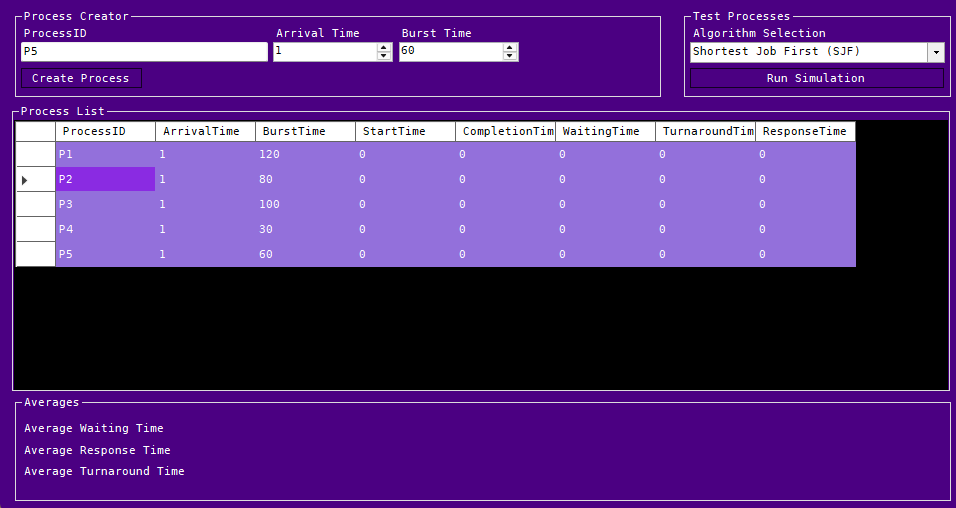
Post Run Conditions:

- Day 9: Implementing Priority Scheduling-
C# - Priority Scheduling
Coding Priority Scheduling as part of the implementation for our simulator in C# for a
WinForms GUI.
Priority Update for Process Class
public class Process
{
    public string ProcessID { get; set; }
    public int ArrivalTime { get; set; }
    public int BurstTime { get; set; }
    public int Priority { get; set; }

    public int StartTime { get; set; }
    public int CompletionTime { get; set; }
    public int WaitingTime { get; set; }
    public int TurnaroundTime { get; set; }
    public int ResponseTime { get; set; }

    public Process(string processId, int arrivalTime, int burstTime, int priority)
    {
        ProcessID = processId;
        ArrivalTime = arrivalTime;
        BurstTime = burstTime;
        Priority = priority;
    }
}
Priority Process Update: The Priority Scheduling requires a simple change to be made to the Process Class, by adding an integer variable for Priority we can now call upon it within the algorithms to schedule processes from the queue.
Priority Scheduling
else if (AlgoComboBox.SelectedItem.ToString() == "Priority")
{
    List queue = new List();
    List remaining = processes.OrderBy(p => p.Priority).ToList();

    int currentTime = 0;

    while (remaining.Count > 0)
    {

        List available = remaining.Where(p => p.ArrivalTime <= currentTime).OrderBy(p => p.Priority).ThenBy(p => p.ArrivalTime).ToList();

        if (available.Count == 0)
        {
            currentTime = remaining.Min(p => p.ArrivalTime);
            continue;
        }

        Process p = available.First();

        p.StartTime = currentTime;
        p.CompletionTime = currentTime + p.BurstTime;
        p.TurnaroundTime = p.CompletionTime - p.ArrivalTime;
        p.WaitingTime = p.TurnaroundTime - p.BurstTime;
        p.ResponseTime = p.StartTime - p.ArrivalTime;

        currentTime = p.CompletionTime;

        queue.Add(p);
        remaining.Remove(p);
    }

    double avgWaitingTime = queue.Average(p => p.WaitingTime);
    double avgTurnaroundTime = queue.Average(p => p.TurnaroundTime);
    double avgResponseTime = queue.Average(p => p.ResponseTime);

    AvgWaitLbl.Text = $"Average Waiting Time: {avgWaitingTime:F2} ms";
    AvgTurnaroundLbl.Text = $"Average Turnaround Time: {avgTurnaroundTime:F2} ms";
    AvgResponseLbl.Text = $"Average Response Time: {avgResponseTime:F2} ms";

    ProcessTabel.DataSource = null;
    ProcessTabel.DataSource = queue;
}
The Priority Scheduling Algorithm: Taking existing code from the Shortest Job First Algorithm, we make a single change to the way ordering is handled in the available process list. Instead of sorting by Burst Time, then Arrival Time. We sort by Priority, then Arrival Time. This ensures any processes arriving within a similar time frame, will process first depending on Priority. As a reminder this is non-preemptive scheduling, so it does not dynamically update priorities, if a process arrives later on. In example, if P1 arrives at 0ms, and has a priority of 1, and P2 arrives at 0 ms with a priority of 2, if P3 arrives before P1 executes fully with a priority of 1, it will not re-order P2 before execution for P3.
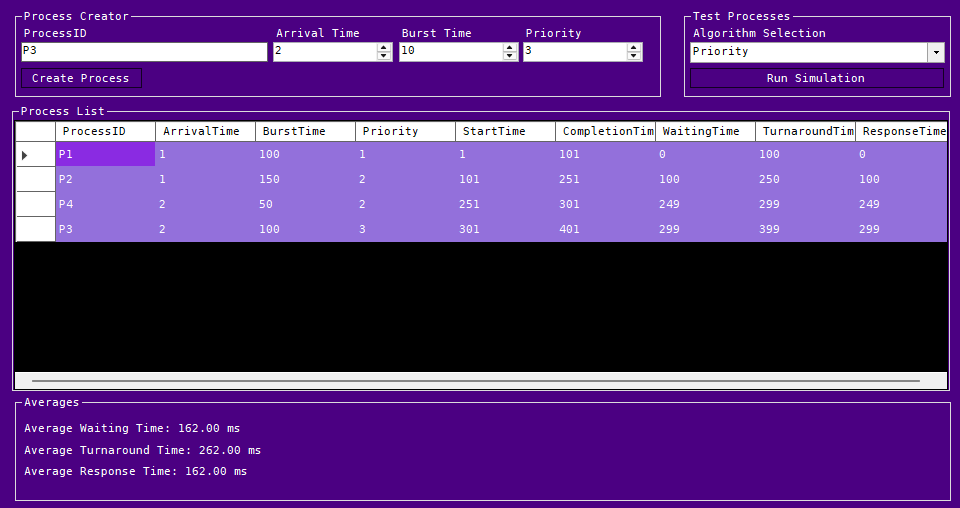
Foot Note
Here we can see the priority scheduling moving Processes based on the Priority Column against Arrival Times.
Priority Simulation:
- Day 10: Implementing Round Robin Scheduling-
C# - Round Robin Scheduling
Coding Round Robin Scheduling as part of the implementation for our simulator in C# for a
WinForms GUI.
Round Robin Update for Process Class
public class Process
{
    public string ProcessID { get; set; }
    public int ArrivalTime { get; set; }
    public int BurstTime { get; set; }
    public int Priority { get; set; }

    public int StartTime { get; set; }
    public int CompletionTime { get; set; }
    public int RemainingTime { get; set; }
    public int WaitingTime { get; set; }
    public int TurnaroundTime { get; set; }
    public int ResponseTime { get; set; }

    public Process(string processId, int arrivalTime, int burstTime, int priority)
    {
        ProcessID = processId;
        ArrivalTime = arrivalTime;
        BurstTime = burstTime;
        Priority = priority;
    }
}
Round Robin Process Update: The Round Robin Scheduling requires a simple change to be made to the Process Class, by adding an integer variable for Remaining Time we can now call upon it within the algorithms to schedule processes from the queue. As seen before with the Priority Variable.
Revision: I've noticed the sorting for the remaining queue was set to Priority rather than Arrival Time; this has been updated and now reflects in the code.
Round Robin Scheduling
else if (AlgoComboBox.SelectedItem.ToString() == "Round Robin (RR)")
{
    int quantum = 15;

    List completedQueue = new List();
    List remaining = processes.OrderBy(p => p.ArrivalTime).ToList();
    Queue readyQueue = new Queue();

    int currentTime = 0;

    foreach (Process p in processes)
    {
        p.RemainingTime = p.BurstTime;
        p.StartTime = -1;
    }

    while (remaining.Count > 0 || readyQueue.Count > 0)
    {
        while (remaining.Count > 0 && remaining.First().ArrivalTime <= currentTime)
        {
            readyQueue.Enqueue(remaining.First());
            remaining.RemoveAt(0);
        }

        if (readyQueue.Count == 0)
        {
            currentTime = remaining.First().ArrivalTime;
            continue;
        }

        Process p = readyQueue.Dequeue();


        if (p.StartTime == -1)
        {
            p.StartTime = currentTime;
            p.ResponseTime = p.StartTime - p.ArrivalTime;
        }

        int runTime = Math.Min(quantum, p.RemainingTime);

        currentTime += runTime;
        p.RemainingTime -= runTime;


        while (remaining.Count > 0 && remaining.First().ArrivalTime <= currentTime)
        {
            readyQueue.Enqueue(remaining.First());
            remaining.RemoveAt(0);
        }

        if (p.RemainingTime > 0)
        {
            readyQueue.Enqueue(p);
        }
        else
        {
            p.CompletionTime = currentTime;
            p.TurnaroundTime = p.CompletionTime - p.ArrivalTime;
            p.WaitingTime = p.TurnaroundTime - p.BurstTime;

            completedQueue.Add(p);
        }

    }

    double avgWaitingTime = completedQueue.Average(p => p.WaitingTime);
    double avgTurnaroundTime = completedQueue.Average(p => p.TurnaroundTime);
    double avgResponseTime = completedQueue.Average(p => p.ResponseTime);

    AvgWaitLbl.Text = $"Average Waiting Time: {avgWaitingTime:F2} ms";
    AvgTurnaroundLbl.Text = $"Average Turnaround Time: {avgTurnaroundTime:F2} ms";
    AvgResponseLbl.Text = $"Average Response Time: {avgResponseTime:F2} ms";

    ProcessTabel.DataSource = null;
    ProcessTabel.DataSource = completedQueue;

}
The Round Robin Algorithm: The Round Robin Algorithm is the first time the algorithm needs to be restructured. First an integer value for the Time Quantum is added then a Queue structure is created. A Queue is different from a List as it removes items from the front and adds them at the end, following First In First Out principles. Then while both the Remaining Process List and Ready Queue contain Processes we begin queuing processes from the Remaining Process List, in to the Ready Queue where it's executed for the time quantum duration, modifying the remaining time. After execution for the time quantum, it's removed from the Ready Queue, and if the Remaining Time is greater than 0, it's re-queued into the Ready Queue.
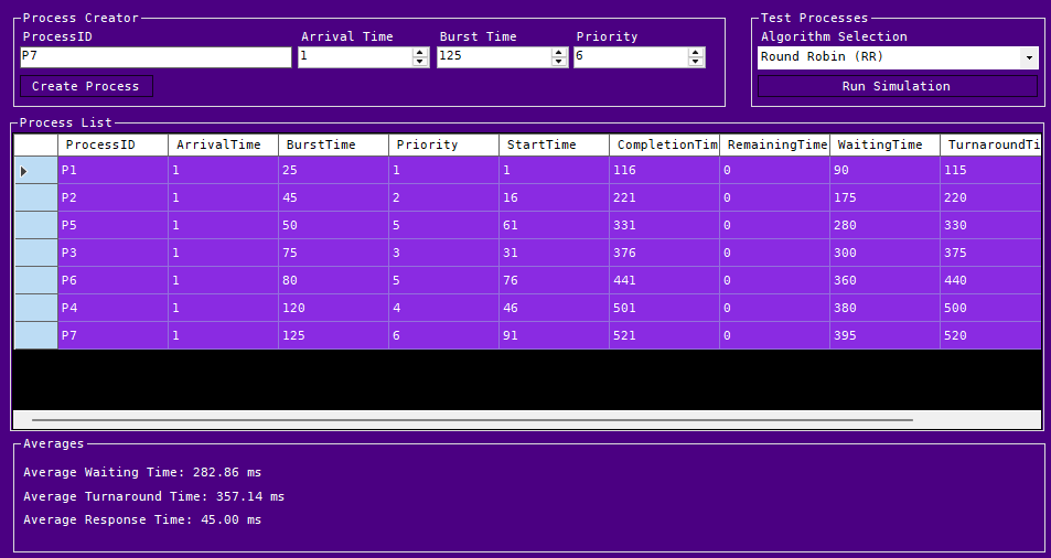
Foot Note
Here we can see the Round Robin Scheduling in effect with the differences in averages, and completion times.
Round Robin Simulation:
- Day 11: Data Set Processing-
Testing larger datasets requires different workloads.
For this, we used ChatGPT to produce three lists of processes. We were able to take the generated
CSVs and import them as processes to run against our algorithms.
Details
Using these datasets required an import function set up with a System.IO and an export function set up with a StreamWriter Object. Below are the files we'll be using.
Process Lists:
Light Load
Medium Load
Heavy Load
Import Button
private void ImportBtn_Click(object sender, EventArgs e)
{
    OpenFileDialog openFileDialog = new OpenFileDialog();
    openFileDialog.Filter = "CSV Files (*.csv)|*.csv";
    openFileDialog.Title = "Import Process List";

    if (openFileDialog.ShowDialog() == DialogResult.OK)
    {
        string[] lines = File.ReadAllLines(openFileDialog.FileName);

        for (int i = 1; i < lines.Length; i++)
        {
            string[] values = lines[i].Split(',');

            string processID = values[0];
            int arrivalTime = int.Parse(values[1]);
            int burstTime = int.Parse(values[2]);
            int priority = int.Parse(values[3]);

            Process newProcess = new Process(
                processID,
                arrivalTime,
                burstTime,
                priority
                );

            processes.Add(newProcess);
        }

        ProcessTabel.DataSource = null;
        ProcessTabel.DataSource = processes;

    }

}
The Import Button: The Import Button is a File Dialog Box that uses System.IO to read each line of a CSV file, using commas as delimiters. From there, variables are set and used as parameters to construct the processes used for data sets.
Export Button
private void ExportBtn_Click(object sender, EventArgs e)
{
    SaveFileDialog saveFileDialog = new SaveFileDialog();
    saveFileDialog.Filter = "CSV Files (*.csv)|*.csv";
    saveFileDialog.Title = "Export Process List";
    saveFileDialog.FileName = "Results.csv";

    if (saveFileDialog.ShowDialog() == DialogResult.OK) {

        using(StreamWriter writer = new StreamWriter(saveFileDialog.FileName))
        {
            writer.WriteLine("ProcessID,ArrivalTime,BurstTime,Priority,StartTime,CompletionTime,WaitingTime,TurnaroundTime,ResponseTime");

            foreach(Process p in processes)
            {

                writer.WriteLine(
                    $"{p.ProcessID}," +
                    $"{p.ArrivalTime}," +
                    $"{p.BurstTime}," +
                    $"{p.Priority}," +
                    $"{p.StartTime}," +
                    $"{p.CompletionTime}," +
                    $"{p.WaitingTime}," +
                    $"{p.TurnaroundTime}," +
                    $"{p.ResponseTime}"
                    );

            }
        }

        MessageBox.Show(
            "Test results exported.",
            "Export Complete",
            MessageBoxButtons.OK,
            MessageBoxIcon.Information
            );

    }
}
The Export Button: The Export Button uses the Save File Dialog Box to save a CSV file containing the test results from the simulation. It uses a StreamWriter Object to write each line consisting of the process characteristics after the simulation runs.
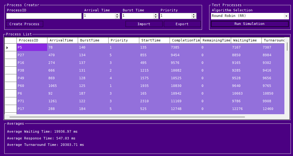
Foot Note
While creating this, I noticed that Round Robin Scheduling was using Priority over Arrival Time. This has since been updated, and it now reflects in Day 10 Notes. The image shows the revised User Interface and an imported data set. From here, we will be working on creating graphs and comparisons within the application itself.
Round Robin Simulation with Heavy Load:
- Day 12: Analysis Part 1 -
Algorithms Analysis - Tables
An initial comparison between the previously constructed algorithms.
Description
For the initial analysis we'll be building tables and looking at the average times between each algorithm. We'll use our application for each workload, and create a comparison set between each workload.
Light Workload : 75 Processes
| Algorithm | Average Wait Time | Average Response Time | Average Turnaround Time |
|---|---|---|---|
| First Come First Served | 13246.69 ms | 13246.69 ms | 13613.43 ms |
| Shortest Job First | 9748.13 ms | 9748.13 ms | 10114.87 ms |
| Priority | 12989.96 ms | 12989.96 ms | 13356.69 ms |
| Round Robin | 19925.71 ms | 1094.23 ms | 20292.44 ms |
Medium Workload : 125 Processes
| Algorithm | Average Wait Time | Average Response Time | Average Turnaround Time |
|---|---|---|---|
| First Come First Served | 26762.13 ms | 26762.13 ms | 27203.93 ms |
| Shortest Job First | 20065.18 ms | 20065.18 ms | 20506.98 ms |
| Priority | 26482.73 ms | 26482.73 ms | 26924.53 ms |
| Round Robin | 40491.44 ms | 1846.21 ms | 40933.24 ms |
Heavy Workload : 200 Processes
| Algorithm | Average Wait Time | Average Response Time | Average Turnaround Time |
|---|---|---|---|
| First Come First Served | 52970.76 ms | 52970.76 ms | 53506.01 ms |
| Shortest Job First | 38893.62 ms | 38893.62 ms | 39428.88 ms |
| Priority | 52769.61 ms | 52769.61 ms | 53304.86 ms |
| Round Robin | 77721.80 ms | 2971.11 ms | 78257.05 ms |
Comparison
Within the tables we can see that the Round Robin algorithm consistently has the lowest average response time, and the longest average wait time and turnaround time. This was expected due to initial estimations previously, as each process has to be visited throughout the queue and is only running against the time quantum. In this case 30 ms was used.
Shortest Job First has the lowest averages across the board, this is again something we can expect with the shorter jobs being executed first from the queue. This would be ideal for batch execution or sequential jobs with start-up processes that execute first with shorter burst times, before lengthier calculations/executions take place.
In this example, First Come First Served and Priority appear to have similar averages. I believe this is due to it being Non-Preemptive Priority Scheduling causing the queue to not dynamically reallocate priority during execution. Once a job comes in it's priority is set until execution completes. This causes the arrival time to play more of a factor over the actual priority of the process.
Foot Notes
When importing workloads I noticed the previous data sets were not clearing. This can be fixed by including, processes.Clear(); at the beginning of the import button function. After adding that I was able to compare the results with out overlap in the working sets.
While reviewing the data I also noticed the Priority Scheduling should be using Priority over Arrival Time and updated the ordering within the code to use OrderBy(p => p.Priority).ThenBy(p => p.ArrivalTime) rather than ArrivalTime first.
- Day 13: Analysis Part 2 -
Algorithms Analysis - Graphs
An secondary comparison between the previously constructed algorithms.
Description
For the secondary analysis we'll be building tables and looking at the average times between each algorithm. We'll build out graphs and charts to visualize the data further. These graphs will be the primary content of these with a comparative analysis below.
Light Workload
Average Wait Time
Average Turnaround Time
Average Response Time
Medium Workload
Average Wait Time
Average Turnaround Time
Average Response Time
Heavy Workload
Average Wait Time
Average Turnaround Time
Average Response Time
Scalability: Average Waiting Time
Comparison
These graphs mirror what we saw previously. Round Robin performs great across the board for Response Times. But fails to maintain performance in Turnaround Time and Wait Time.
Shortest Job First has the lowest average, with the shortest jobs executed first from the queue. This is reflected again in both the bar charts and the scalability graph. Leading thought that, in terms of Non-Preemptive Scheduling, it's the best option.
We can still see the First Come First Served and Priority Algorithms mirroring each other almost identically. Either being a good fit when comparing averages.
Foot Notes
For clarity, the research project is coming to a close. With the information we have here, we can now draft a final report on Non-Preemptive Scheduling Algorithms and close out this initial item. Thank you for joining me on this journey. Day 14 will consist of an outline identifying points for the final entry on Day 15.
- Day 14: Outline -
Defining the Outline
A final report should follow guidelines and a format that allow for the citation of sources and the condensation of knowledge.
Abstract
Here we'll identify the points of the study subject. Our purpose: Why did we do this research? What do we gain from it? Algorithm designs: What algorithms did we choose? How did we compare them? Simulator Design: Why was it created? What purpose did it serve? Workloads Tested: The original choices? Are we testing more? Primary Findings: What did we learn?
Introduction
Our introduction will cover what CPU Scheduling is and why it exists. Alongside why it matters in Operating Systems. We'll ask questions and record the answers we find. Lastly, we'll identify the research goals.
Background
Within the background section, we'll outline the topics covered within the research itself. CPU Scheduling, First Come First Served, Shortest Job First, Round Robin, and Priority Scheduling. We'll summarize key findings for each piece and the purpose each serves.
Methodology
Here we'll cover the method used to perform research, why we chose C# to build the simulator alongside why we gave it a GUI. The process class and why it was built the way it was. Revisit the algorithms we chose and why, alongside the datasets we used, and any additional data sets we built. We'll then outline the metrics collected and purpose they served.
Implementation and Results
For implementation and results, we'll revisit and outline the steps taken during the initial setup of each algorithm, the process class we built, the validation we used to identify errors, and the test cases we used. Additionally, we'll include tables, graphs, and average comparisons against the original datasets and any other datasets we test against.
Discussion
Before the conclusion, we'll identify the areas of interest from the research and ask why. For example, Why did SJF perform best? Why was RR slower? Why were First Come First Served and Priority similar? How did workload size affect performance? Would these results change in real operating systems?
Conclusion
With the conclusion we'll identify if the research provided any tangible results, what we would do differently if we performed this research again, and what we learned from it.
Footnote
As this project was intended to be a self study preparation, we won't be peer reviewing this. We'll aim for 2500-3000 words, focusing on the subject of CPU Scheduling. Identifying weak points, and area's we can improve critically after the conclusion. With the intent of this site to develop a skill set in Generative AI, HTML, CSS, and a small bit of JavaScript. We've been using ChatGPT, Youtube Videos, and W3Schools to design and implement the majority of what you see on screen.
- Day 15: Conclusions -
New Beginnings
Concluding our research with a final entry following the previous days outline.
Abstract
To facilitate understanding of CPU Scheduling and how processes operate on threaded CPUs, we began a short 15-day study of CPU Scheduling Algorithms and their operation in modern operating systems. Our intended purpose was to prepare for future study and self-paced projects. We gained a deeper understanding of these Algorithms, experimented with prompt engineering alongside ChatGPT, and gained some C# experience inside of Visual Studio.
In this study session, we chose to proceed with non-preemptive algorithms, specifically first-come, first-served, shortest-job-first, round-robin, and priority scheduling. The choice was made based on our experience level: the foundational programming skills were present, but self-paced research and higher-level functional skills were not. We compared them using the essential direct comparison of averages to see how they would perform under specific conditions and where they would excel.
Alongside this, a simulation program was created, which was bare-bones and simply ran functions against a single class. It still implemented object-oriented principles, used system classes, and provided a stepping stone for future projects. We’ve used it for the initial analysis of each algorithm and will use it again later in this paper to compare additional datasets.
With this, the datasets used consist of a light workload (75 processes), a medium workload (125 processes), and a heavy workload (200 processes). These allow us to see the gradual onset scaling effects of each process and how the CPU's overall workload increases as the workload increases.
The primary results yielded simple returns and an interesting understanding of which algorithm is best suited to specific computational conditions. For example, batch processing may be best suited to Shortest Job First if burst times are known for each case. If a linear computational process is needed, First-Come First-Served is better suited. While a real-time or interactive system, depending on the use case, may be better suited for Priority Scheduling or the Round Robin algorithm.
Introduction
The importance of CPU Scheduling lies in the fact that modern operating systems react to your input, with too much latency, we lose the impact or sense of freedom that the historical progress of computational science has provided us with the quality of life we have today. Specifically, CPU Scheduling is a fundamental function of an operating system that allocates the CPU among multiple processes competing for execution. Because CPU cores can handle only a single process at a time, scheduling ensures they operate with minimal latency.
CPU Scheduling is essential for real-time response and multitasking, which are features of all modern operating systems. They also play a crucial role in resource distribution and load balancing, enabling multiple users to share the system effectively.
Our initial question was simple: What is CPU Scheduling? The above section answers that for us. Our next question began very simply: How does it all work? From that question, we followed through multiple online sources. We asked our readily available chatbot for further clarification if we couldn’t understand. While it appears simple at the top level, it’s a multifaceted operation that follows multiple bridged paths. Depending on the resources in use, the context-switching needed, the queue, the algorithm in use, and, lastly, the desired outcome. All these variables play into which algorithm is in use and how it works effectively in the system at hand.
As previously mentioned, this research was strictly for fun, to develop a skill set for self-managed self-study, and something to do on Khonsu. While the material here may not be perfect, as with everything, it should be fact-checked and verified by an expert when needed.
Background
As described above, CPU Scheduling is essential to modern-day operating systems and has a vital role in the quality of life technology employs today.
The First Come, First Served algorithm is a simple queue that operates on the First-In, First-Out principle, sorting simply by arrival time.
In the Shortest Job First algorithm, burst times are desirable when known. If they are unknown, an estimate must be made. Once they are known or an estimate is made, the algorithm will order them by arrival time, then by burst time. So that shorter jobs go first, as the name implies.
Round Robin operates on a concept known as a time quantum, or time segment, where each process in the queue visits the CPU and receives resources for the set time quantum, at which point it is re-queued at the back of the queue until completion. Round Robin visits each process once until all processes in the queue are completed.
Lastly, Priority Scheduling functions on the priority designated to the process. It depends entirely on the system at hand; in a manufacturing-oriented system, the principle of safety may prioritize completion, so if a system is working through a sequence of processes and an urgent-priority process arrives as a failsafe, it will execute that next.
Each of these functions operates differently, depending on whether it is preemptive or non-preemptive. This study was conducted on non-preemptive algorithms, and it must be noted that all previous sections and all sections of this paper reflect that.
Methodology
Our methodology was based on learning and implementation. We read a subject, described the process, and attempted to produce tangible results in Visual Studio, with ChatGPT double-checking our work and grading each day's material against an undergraduate study baseline. We built the simulator in C# WinForms because it was the most recent application type I had developed.
After identifying the primary components of the process class, for example, the bare minimum needed to develop a simulation, we took the time to build it out as a class. With this, we identified the need for a Process ID, Burst Time, Arrival Time, and Priority. From there, we added additional properties for Start Time, Completion Time, Response Time, Remaining Time, Waiting Time, and Turnaround Time. We deviated from the original outline because the need for Booleans was not necessary for the algorithms' execution.
From there, we outlined what was needed to return metrics for each process, against Waiting Time, Turnaround Time, and Response Time. After we looked at how to store the processes and execute them within the queue. We built algorithms for First Come First Served, where we took the processes created by the user, sorted them by arrival time, and executed them in the order of arrival. Using the C# Math function for Averages to view Average Wait Time, Average Turnaround Time, and Average Response Time.
Next, we built out the Shortest Job First Algorithm. Because it is non-preemptive, we first sorted by arrival time, then filtered by burst time and arrival time, adding each to a queue of available processes. The first available process was executed based on arrival time and burst time.
With Priority Scheduling, we originally sorted by arrival time, then by priority. Which was incorrect; we have since corrected it to sort by priority, then arrival time. We followed a similar principle to Shortest Job First, creating a queue of remaining and available processes to execute, then sorting and selecting the first available process.
For Round Robin, we used the processes and set the remaining time to the full burst time, then followed the same principles as in both Shortest Job First and Priority Scheduling. Here, we used a Queue Object rather than a List Object, where processes were added to the remaining list, enqueued into the queue object, executed, and then removed before being added again until completion. Once the process was completed, it was then added to a second list, the Completed Queue.
After the research and implementation were completed, an import button was created alongside the three initial datasets, generated by ChatGPT, to run against the application itself. From there, we recorded data and created Days 12 and 13 entries consisting of the average results and observed comparisons.
Implementation and Results
Here we will look at previous entries sorted in descending order of code blocks, tables, and then graphs.
The Process Class
public class Process
{
    public string ProcessID { get; set; }
    public int ArrivalTime { get; set; }
    public int BurstTime { get; set; }

    public int StartTime { get; set; }
    public int CompletionTime { get; set; }
    public int WaitingTime { get; set; }
    public int TurnaroundTime { get; set; }
    public int ResponseTime { get; set; }

    public Process(string processId, int arrivalTime, int burstTime)
    {
        ProcessID = processId;
        ArrivalTime = arrivalTime;
        BurstTime = burstTime;
    }
}
The Process Class: The Process Class is implemented here, with variables, set, and get, for Process IDs, Arrival Times, Burst Times (Execution Times), Start Times, Completion Times, Wait Times, Turnaround Times, and Response Times. With a Constructor for a Process, consisting of Process ID's, Arrival Times, and Burst Times (Execution Times), with this being the first iteration, and pertaining to First Come First Serve, we kept it simple without any additional variables.
The First Come First Serve Simulation
    if (AlgoComboBox.SelectedItem == "First Come First Serve (FCFS)")
    {
        List queue = processes.OrderBy(p => p.ArrivalTime).ToList();

        int currentTime = 0;

        foreach (Process p in queue)
        {
            if (currentTime < p.ArrivalTime)
                currentTime = p.ArrivalTime;

            p.StartTime = currentTime;
            p.CompletionTime = currentTime + p.BurstTime;
            p.TurnaroundTime = p.CompletionTime - p.ArrivalTime;
            p.WaitingTime = p.TurnaroundTime - p.BurstTime;
            p.ResponseTime = p.StartTime - p.ArrivalTime;

            currentTime = p.CompletionTime;
        }
    }
The First Come First Serve Simulation: This button begins the simulation. By using the global process list, we order the Processes by Arrival Time in the Queue. After confirming the selected algorithm from our combobox, we start the simulation. For each process in the queue, we check if the Current Time is less than the Arrival time. If it is we set the Current Time to the Arrival Time. After we set the process Start Time to the Current Time. Calculate the Completion Time by adding the Burst Time to the Current Time within the simulation. Then calculate the Turnaround Time by subtracting the Arrival Time, from the Completion Time. The Wait Time is calculated by subtracting the Burst Time from the Turnaround Time. Then the Response Time is set by subtracting the Arrival Time from the Start Time. We then set the Current Time to the Completion Time for the process in the queue.
Shortest Job First
else if (AlgoComboBox.SelectedItem.ToString() == "Shortest Job First (SJF)")
{
    List queue = new List();
    List remaining = processes.OrderBy(p => p.ArrivalTime).ToList();

    int currentTime = 0;

    while (remaining.Count > 0)
    {

        List available = remaining.Where(p => p.ArrivalTime <= currentTime).OrderBy(p => p.BurstTime).ThenBy(p => p.ArrivalTime).ToList();

        if (available.Count == 0)
        {
            currentTime = remaining.Min(p => p.ArrivalTime);
            continue;
        }

        Process p = available.First();

        p.StartTime = currentTime;
        p.CompletionTime = currentTime + p.BurstTime;
        p.TurnaroundTime = p.CompletionTime - p.ArrivalTime;
        p.WaitingTime = p.TurnaroundTime - p.BurstTime;
        p.ResponseTime = p.StartTime - p.ArrivalTime;

        currentTime = p.CompletionTime;

        queue.Add(p);
        remaining.Remove(p);
    }
}
The Shortest Job First Algorithm: Combining existing code from the First Come First Served Algorithm, we then add two new lists for Available Processes, and Remaining Processes, Ensuring the Arrival Time is less than or equal to the Current Time, we order by Burst Time (Execution Time) and Arrival Time. To ensure fairness if two jobs of similar lengths arrive between execution of the current process. If the available processes run out, we grab the last remaining process, and execute it from its arrival time.
Priority Update for Process Class
public class Process
{
    public string ProcessID { get; set; }
    public int ArrivalTime { get; set; }
    public int BurstTime { get; set; }
    public int Priority { get; set; }

    public int StartTime { get; set; }
    public int CompletionTime { get; set; }
    public int WaitingTime { get; set; }
    public int TurnaroundTime { get; set; }
    public int ResponseTime { get; set; }

    public Process(string processId, int arrivalTime, int burstTime, int priority)
    {
        ProcessID = processId;
        ArrivalTime = arrivalTime;
        BurstTime = burstTime;
        Priority = priority;
    }
}
Priority Process Update: The Priority Scheduling requires a simple change to be made to the Process Class, by adding an integer variable for Priority we can now call upon it within the algorithms to schedule processes from the queue.
Priority Scheduling
else if (AlgoComboBox.SelectedItem.ToString() == "Priority")
{
    List queue = new List();
    List remaining = processes.OrderBy(p => p.Priority).ToList();

    int currentTime = 0;

    while (remaining.Count > 0)
    {

        List available = remaining.Where(p => p.ArrivalTime <= currentTime).OrderBy(p => p.Priority).ThenBy(p => p.ArrivalTime).ToList();

        if (available.Count == 0)
        {
            currentTime = remaining.Min(p => p.ArrivalTime);
            continue;
        }

        Process p = available.First();

        p.StartTime = currentTime;
        p.CompletionTime = currentTime + p.BurstTime;
        p.TurnaroundTime = p.CompletionTime - p.ArrivalTime;
        p.WaitingTime = p.TurnaroundTime - p.BurstTime;
        p.ResponseTime = p.StartTime - p.ArrivalTime;

        currentTime = p.CompletionTime;

        queue.Add(p);
        remaining.Remove(p);
    }

}
The Priority Scheduling Algorithm: Taking existing code from the Shortest Job First Algorithm, we make a single change to the way ordering is handled in the available process list. Instead of sorting by Burst Time, then Arrival Time. We sort by Priority, then Arrival Time. This ensures any processes arriving within a similar time frame, will process first depending on Priority. As a reminder this is non-preemptive scheduling, so it does not dynamically update priorities, if a process arrives later on. In example, if P1 arrives at 0ms, and has a priority of 1, and P2 arrives at 0 ms with a priority of 2, if P3 arrives before P1 executes fully with a priority of 1, it will not re-order P2 before execution for P3.
Round Robin Update for Process Class
public class Process
{
    public string ProcessID { get; set; }
    public int ArrivalTime { get; set; }
    public int BurstTime { get; set; }
    public int Priority { get; set; }

    public int StartTime { get; set; }
    public int CompletionTime { get; set; }
    public int RemainingTime { get; set; }
    public int WaitingTime { get; set; }
    public int TurnaroundTime { get; set; }
    public int ResponseTime { get; set; }

    public Process(string processId, int arrivalTime, int burstTime, int priority)
    {
        ProcessID = processId;
        ArrivalTime = arrivalTime;
        BurstTime = burstTime;
        Priority = priority;
    }
}
Round Robin Process Update: The Round Robin Scheduling requires a simple change to be made to the Process Class, by adding an integer variable for Remaining Time we can now call upon it within the algorithms to schedule processes from the queue. As seen before with the Priority Variable.
Revision: I've noticed the sorting for the remaining queue was set to Priority rather than Arrival Time; this has been updated and now reflects in the code.
Round Robin Scheduling
else if (AlgoComboBox.SelectedItem.ToString() == "Round Robin (RR)")
{
    int quantum = 15;

    List completedQueue = new List();
    List remaining = processes.OrderBy(p => p.ArrivalTime).ToList();
    Queue readyQueue = new Queue();

    int currentTime = 0;

    foreach (Process p in processes)
    {
        p.RemainingTime = p.BurstTime;
        p.StartTime = -1;
    }

    while (remaining.Count > 0 || readyQueue.Count > 0)
    {
        while (remaining.Count > 0 && remaining.First().ArrivalTime <= currentTime)
        {
            readyQueue.Enqueue(remaining.First());
            remaining.RemoveAt(0);
        }

        if (readyQueue.Count == 0)
        {
            currentTime = remaining.First().ArrivalTime;
            continue;
        }

        Process p = readyQueue.Dequeue();


        if (p.StartTime == -1)
        {
            p.StartTime = currentTime;
            p.ResponseTime = p.StartTime - p.ArrivalTime;
        }

        int runTime = Math.Min(quantum, p.RemainingTime);

        currentTime += runTime;
        p.RemainingTime -= runTime;


        while (remaining.Count > 0 && remaining.First().ArrivalTime <= currentTime)
        {
            readyQueue.Enqueue(remaining.First());
            remaining.RemoveAt(0);
        }

        if (p.RemainingTime > 0)
        {
            readyQueue.Enqueue(p);
        }
        else
        {
            p.CompletionTime = currentTime;
            p.TurnaroundTime = p.CompletionTime - p.ArrivalTime;
            p.WaitingTime = p.TurnaroundTime - p.BurstTime;

            completedQueue.Add(p);
        }

    }

}
The Round Robin Algorithm: The Round Robin Algorithm is the first time the algorithm needs to be restructured. First an integer value for the Time Quantum is added then a Queue structure is created. A Queue is different from a List as it removes items from the front and adds them at the end, following First In First Out principles. Then while both the Remaining Process List and Ready Queue contain Processes we begin queuing processes from the Remaining Process List, in to the Ready Queue where it's executed for the time quantum duration, modifying the remaining time. After execution for the time quantum, it's removed from the Ready Queue, and if the Remaining Time is greater than 0, it's re-queued into the Ready Queue.
Process Lists:
Light Load
Medium Load
Heavy Load
Light Workload : 75 Processes
| Algorithm | Average Wait Time | Average Response Time | Average Turnaround Time |
|---|---|---|---|
| First Come First Served | 13246.69 ms | 13246.69 ms | 13613.43 ms |
| Shortest Job First | 9748.13 ms | 9748.13 ms | 10114.87 ms |
| Priority | 12989.96 ms | 12989.96 ms | 13356.69 ms |
| Round Robin | 19925.71 ms | 1094.23 ms | 20292.44 ms |
Medium Workload : 125 Processes
| Algorithm | Average Wait Time | Average Response Time | Average Turnaround Time |
|---|---|---|---|
| First Come First Served | 26762.13 ms | 26762.13 ms | 27203.93 ms |
| Shortest Job First | 20065.18 ms | 20065.18 ms | 20506.98 ms |
| Priority | 26482.73 ms | 26482.73 ms | 26924.53 ms |
| Round Robin | 40491.44 ms | 1846.21 ms | 40933.24 ms |
Heavy Workload : 200 Processes
| Algorithm | Average Wait Time | Average Response Time | Average Turnaround Time |
|---|---|---|---|
| First Come First Served | 52970.76 ms | 52970.76 ms | 53506.01 ms |
| Shortest Job First | 38893.62 ms | 38893.62 ms | 39428.88 ms |
| Priority | 52769.61 ms | 52769.61 ms | 53304.86 ms |
| Round Robin | 77721.80 ms | 2971.11 ms | 78257.05 ms |
Comparison
Within the tables we can see that the Round Robin algorithm consistently has the lowest average response time, and the longest average wait time and turnaround time. This was expected due to initial estimations previously, as each process has to be visited throughout the queue and is only running against the time quantum. In this case 30 ms was used.
Shortest Job First has the lowest averages across the board, this is again something we can expect with the shorter jobs being executed first from the queue. This would be ideal for batch execution or sequential jobs with start-up processes that execute first with shorter burst times, before lengthier calculations/executions take place.
In this example, First Come First Served and Priority appear to have similar averages. I believe this is due to it being Non-Preemptive Priority Scheduling causing the queue to not dynamically reallocate priority during execution. Once a job comes in it's priority is set until execution completes. This causes the arrival time to play more of a factor over the actual priority of the process.
Light Workload
Average Wait Time
Average Turnaround Time
Average Response Time
Medium Workload
Average Wait Time
Average Turnaround Time
Average Response Time
Heavy Workload
Average Wait Time
Average Turnaround Time
Average Response Time
Comparison
These graphs mirror what we saw previously. Round Robin performs great across the board for Response Times. But fails to maintain performance in Turnaround Time and Wait Time.
Shortest Job First has the lowest average, with the shortest jobs executed first from the queue. This is reflected again in both the bar charts and the scalability graph. Leading thought that, in terms of Non-Preemptive Scheduling, it's the best option.
We can still see the First Come First Served and Priority Algorithms mirroring each other almost identically. Either being a good fit when comparing averages.
Discussion Why did SJF perform best?
Shortest Job First performed better in this simulation simply because the burst times were known. In a real-world situation where burst times must be estimated dynamically, there is no guarantee that Shortest Job First would be beneficial. Unless, in a situation where the burst times were known in advance, for example, a batch processing operation with startup processes that were shorter than the calculations taking place.
Why was RR slower?
Round Robin was slower because it split each process into multiple slices against the time quantum. To facilitate the algorithm's execution against each process segmented into n time slices, it simply takes longer.
Why were First Come First Served and Priority similar?
First Come First Served and Priority appear similar because the arrival time of the process plays a role in execution. With priority and first-come, first-served, they are sorted by arrival time. Within the arrival time window, they are ordered by priority, meaning it still starts as first-come, first-served before the priority order.
How did workload size affect performance?
Workload size directly affected performance, increasing the duration of work.
Would these results change in real operating systems?
Yes, in a real-world operating system, unless the algorithms are implemented as non-preemptive versions with the same conditions for the processes, this would function differently, as hardware has physical constraints such as voltage and temperature. And more so, clock speed, memory speed, and resource use directly affect the CPU's processing speed against kernel instructions rather than in a simulated environment.
Conclusion
At the end, the research provided a basic understanding of CPU Scheduling and its purposes, as well as where each algorithm would be a good fit. If I ever need to build a real-time mission-critical operating system that dynamically calculates hundreds of processes at once. I know I should have two processing units. One that uses a combination of preemptive priority and round-robin.
Since that is far in the distant future and outside my current skill set. We’ll take time to reflect on what we would do differently. If this research were performed again, I would include additional datasets. I would include both preemptive and non-preemptive algorithms, as well as a conductor to assist in managing processes, just to learn how to. Nonetheless, it was an enjoyable lesson and taught the very basics of CPU Scheduling.
Sources
External Links - You're leaving Khonsu!
Geeks for Geeks, Preemptive and Non-Preemptive SchedulingGeeks for Geeks, CPU Scheduling in Operating Systems
IntelliPaat, CPU Scheduling in Operating Systems
Wikipedia, Scheduling(Computing)
Farewells
While we didn't quite reach our goal of 2500 words, we reached 1600. Thank you for taking the time to read through this, we appreciate the visits.